-- Flandrin and Martin, 1997
[Case's Homepage] | [Test Signal Page] | [Case's Posters (1906 Centennial Conference)]
[April 2006] Link added to the posters/paper I presented at the 1906 earthquake centennial conference, 18-21 April, 2006, San Francisco. 1906 Conference Posters/Paper. These posters summarize some of my Time-Frequency work, and demonstrate some of the advantages of the Wigner-Ville Distribution (and related quadratic TFR methods).
[Oct 2005] [Test Signal Page added] I have added a link to some example pages. I first create a test signal, and then show the results of various TFR techniques for the same signal, to demonstrate common sources of interference. As always, e-mail me if you have any questions.
In this page I will introduce some concepts related to Time-Frequency representations of non-stationary signals. The first such representation is the "Wigner-Ville Distribution" (or "Wigner-Ville Spectrum") which is functionally similar to a spectrogram. On the whole it gives better temporal and frequency resolution, at the expense of many artifacts and the introduction of negative values, which would correspond to negative energy (this is not physically possible, and represents a significant defect in this method). These are known issues with the W-V spectrum, and there are ways to compensate. You can see that even with these artifacts, the W-V spectrums I show below have very useful information, more so than the spectrograms that I use for comparison. For some of these figures I have taken the absolute value of the W-V spectrum -- these plots show a little more detail as to how the energy is distributed.
For a spectrogram, the dimension of your result (a 2-D matrix) remains constant -- generally speaking, if you increase your resolution in the time domain it comes at the cost of a loss of resolution in frequency.... I think of it as long skinny rectangles or short fat ones. When making my plots I usually create a few spectrograms at different windowing resolutions to compensate for this. It is also possible to perform a spectrogram using a sliding window on a point-by-point basis, but this does not reduce the inherent uncertainty in the method; the length of the window will by definition smear information in the time axis, and the length is inversely proportional to the resolution in the frequency domain.
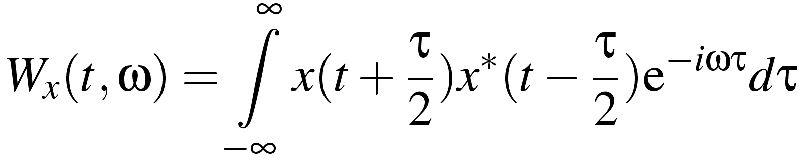
For a signal, s(t), with analytic associate x(t), the Wigner-Ville Distribution, Wx(t,ω) is defined as:
|
|
| Wigner Ville Distribution - notice that it is "FFT-like" in general form. |
| "...a Fourier Transform acting on the delay variable of a properly symmetrized (with respect to evaluation time) covariance function." -- Flandrin and Martin, 1997 |
In general the 'Wigner Distribution' of a signal x(t) is defined as above, while the 'Wigner-Ville Distribution' is defined as the Wigner Distribution where x(t) is the analytic associate (also "analytic signal" or "complex signal") of s(t). The analytic associate x(t) of a signal s(t) is defined as x(t)=s(t)+iH[s(t)], where H[s(t)] is the Hilbert Transform of the signal s(t); the Hilbert Transform is sometimes referred to as a "quadrature filter" and the transformed signal as the "quadrature signal," for reasons relating to the phase shifts introduced by the transform -- running the transform four times will return the signal to the original signal, as each transformation shifts real frequencies by π/2 and negative frequencies by -π/2. In these pages I will be referring to TFR techniques applied to the analytic associates of real signals -- in particular, x(t) is generally the complex-valued analytic associate of some real-valued time signal of interest.
This distribution was first introduced by E. Wigner in the context of quantum mechanics (Wigner, 1932), and later independently developed by J. Ville who applied the same transformation to signal processing and spectral analysis (Ville, 1948).
For the W-V spectrum, I can theoretically create a distribution with as many points in the time domain as there are in the original time series, while simultaneously having the same resolution in the frequency domain! The trade-offs include: the numerical and implementation issues I mentioned above; artifacts along frequency axis from harmonics or more than one peak; the generation of negative energy; artifacts along time axis if you have multiple "events" in time... say an earthquake and an aftershock in the same record, or even multiple phases arriving from the same event.
 |
Chirp function, Wigner-Ville (TOP) and Spectrogram (BOTTOM) Comparison Note the artifacts. This signal also generates negative energy, plots are of log10(abs(Wigner-Ville)). This plot suffers from a type of complicated aliasing that wraps in both the time and frequency axes. [UPDATE: ERROR ALERT] I incorrectly took the W-V transform of a real-valued signal, when the function was expecting the analytic associate of this same signal. Corrected plot below. I leave this here as a cautionary example - if your output looks like this, you've probably made a similar error. |

| Corrected This is very nice, exactly what we'd expect. Problems include a small amount of noise coming in underneath the signal (clearer in log plot) and also negative energy along the line. |

| Corrected (Log10(abs( ))) The interference terms are showing up more clearly now. |
 |
Here's what the chirp looks like |
 |
RID of sine wave with one missing point Missing point is at 666, the RID representation of the glitch is showing up like expected. The extra frequency content is "smeared" out for a short distance, but the RID is able to identify the correct time instant of the missing point. |
 |
Same, linear scale. I adjusted the colormap, as otherwise the glitch response is difficult to resolve. |
[A time-summation of the WVD and the FFT. (From Parkfield, above.)]
 Time summation of WVD and Fourier Transform.
This shows that the WVD does not impose large net negative energy... There are a few spectral holes, but only in places that have low energy as shown in the FT.
The time summation is the sum of all columns of the WV spectrum. The FT is the standard FT of the event, tapered at the ends. This helps justify "smoothing" of the WV distribution, as we see in the Reduced Interference Distribution below. The WW Spectrum, in fact, satisfies the so called 'marginal conditions', in that the integral along the time axis is exactly the Power Spectrum (FT squared) of the signal -- in this case my implementation was for a coarse sampling interval, so the time-summation does not give the exact Fourier spectrum. [EDIT OCT 7] ...and, of course, this should compare the FT squared with the sum along the time axis, expect an update shortly.
The reduced interference distribution has some advantages over a standard Wigner-Ville spectrum. They are both time-frequency distributions in the same family (Cohen's general class) but some previous research has shown the RID to be better suited to the transient signals we see during earthquake events.
(In general, a "Reduced Interference Distribution" refers to any distribution that reduces the expression of the cross-terms relative to the auto-terms in a quadratic TFR representation -- the RID distribution given here is one particular member of a broad class of such representations.)
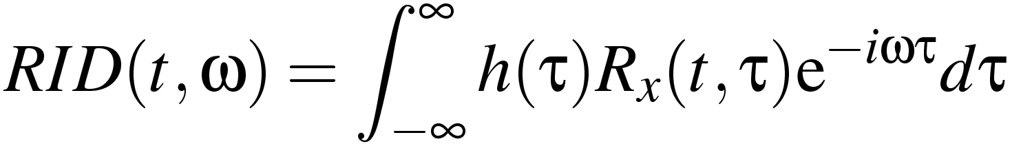
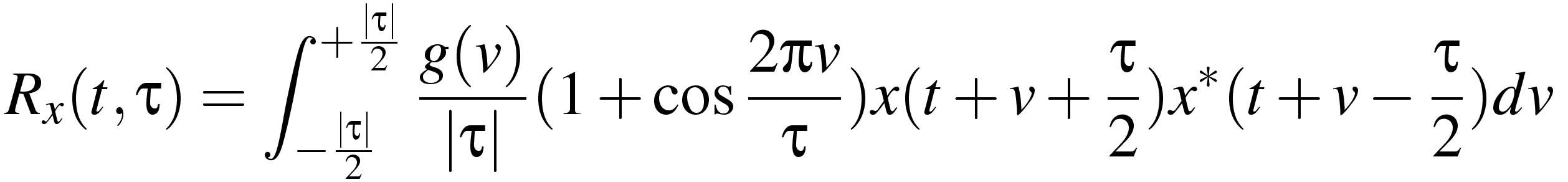
The Reduced Interference Distribution, RID(t,ω) with kernel Rx(t,τ) based on a time series s(t) with analytic associate x(t):
|
| Reduced Interference Distribution - note similarity to WVD in general form, with addition of smoothing kernel in Rx: |
|
| ...h(τ) is a time smoothing window, and g(ν) is a frequency smoothing window. When using Time-Frequency analysis packages these parameters are adjustable depending on your windowing and smoothing needs, see the links section for some packages with RID implementations. In this case I have presented a RID formulation for a Hanning window of [(1 + cos(2πν/τ))/2], but other common smoothing kernels include binomial, bessel and triangular (or "bartlett") windows. For different choices of kernel, the formulation of Rx(t,τ) will change, but it will retain its general auto-correlation structure. |
Mathematically, the RID is a "smoothed" WVD. A particular type of interference, that from cross-terms, tends to be oscillatory, so applying a simple filter (smoothing with a boxcar) can reduce the effect of this interference. I have looked at smoothing in both the time and frequency axes, and doing first one, then the other in either order. The RID applies a 2-D simultaneous filter, it can be thought of as a top hat, the exact shape of which is determined by the choice of smoothing kernel.
I have a few RID plots from the same earthquake as above, as well as testing it on a summation of chirp functions and comparisons with the standard WVD and spectrograms.
 |
Double Chirp Function A good test function for picking peaks of wandering frequencies. Sample Matlab script to generate this signal is available in downloads below. |
 |
Spectrogram and WVD of this chirp Neither gets it right -- the spectrogram is blocky and the WVD has some interference terms between the two signals. (Note the oscillatory nature of the interference terms.) |
 |
RID and WVD of this chirp The RID has a much clearer picture of what is going on -- very close to the "right" answer. The interference is magnitudes smaller (clearer to see on the next plot). |
 |
2-D and 3-D Plots of RID and WVD These show the improvements of RID over WVD. In the 3-D plot you can more easily see the difference in relative amplitude of the interference caused by cross terms in the WVD. |
 |
RID for Parkfield, log10(abs( )). I have again taken the absolute value of the distribution. The RID did not remove the negative values as clearly as I had hoped, so this is still an approximation for the instantaneous energy. |
 |
The same, for [0-10Hz] This method is too numerically intensive to run on the 80sps data, so I used the 20sps data instead. |
 |
Linear scaling, no absolute value. |
 |
Linear scaling, no abs, for [0-10Hz]. |
This page was initially written for internal use, so I've been lax on my citations. In this section I will try to provide some useful references, including some of the papers that I have found useful in the above work.
I also have some posters/presentations at my presentations page, including some posters from the 1906 Centennial Earthquake Conference which can be found here.
REFERENCES (Not in alphabetical order.)
|


