[Case Main TFR Page] | [Simple TFR Method]
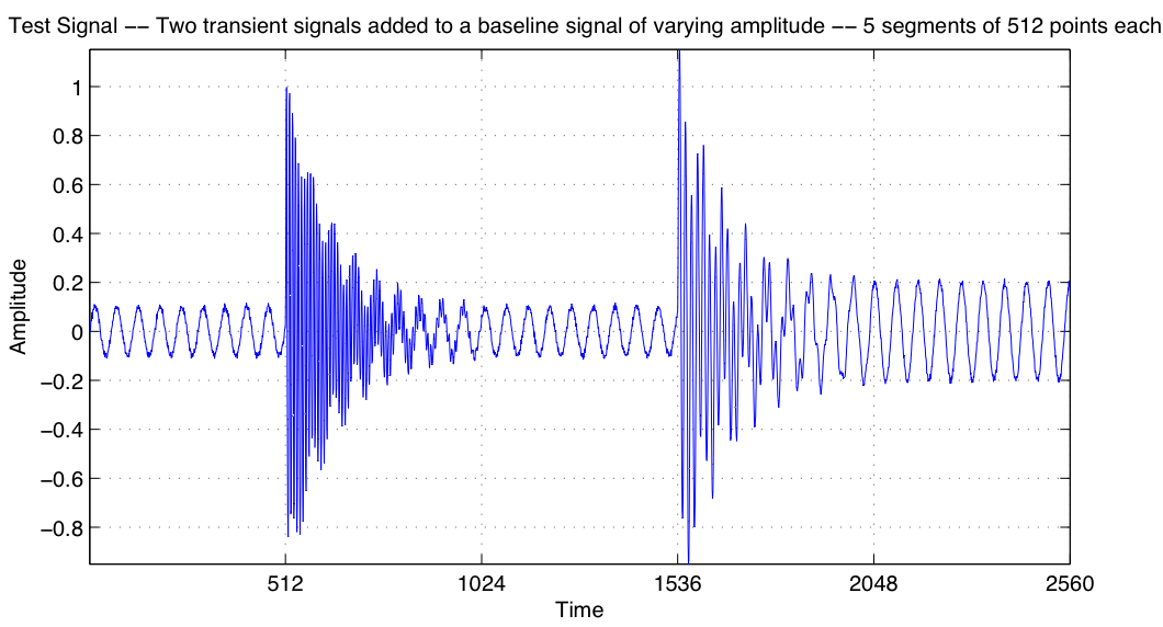
The test signal in this case is broken into 5 main pieces of 512 points each, for a total length of 5*512=2560:
This test signal was created to roughly match an example case given in Leonowicz, et al., 2003 [references below].
|
This page is an update to my previous page on this 2D filter method, which is still available here.
[Sept 22] I've added log plots of these distributions, which shows more clearly the location of energy in the TF plane. I also corrected a problem with the scalogram plot, and applied it as a 2-D overlay to the WVD. Again, in general, I think that the kernel-smoothing done by other modern methods (RID, Choi-Williams, ZAM) does a better job of removing the cross term interference, though these methods do still have problems with positivity and time/frequency resolution.
[Sept 30] It's probably also useful to note that the "2-D Overlay" filtering that I've been developing has already been discovered under the name of the "Masked WVD" according to "Time Frequency Signal Analysis and Processing: A Comprehensive Reference," B. Boashash (ed.), 2003 [references below]. This Masked WVD is exactly the use of the spectrogram as an overlay for the WVD -- and the consensus in the literature is that it is more effective to eliminate cross-term interference in the integral, than to try and remove it with a filter/overlay afterwards. For a simple example of why this would be the case, you only need to imagine a sample signal as below (composed of transient A and B), but with an additional signal component (C) located between the two transient signals in the T-F plane. There would be no straightforward way to separate out the cross terms from A and B without damaging the character of the auto terms from signal C. We approach this case in the Morlet overlay plots below, where the cross terms from the baseline signal and the high-frequency transient impinge on the middle-frequency transient, and are correspondingly included even in the "wavelet-masked" version. In the seismic signals of interest to Civil Engineering, we will often have many closely spaced components of the signal, which makes the masked/overlay methods less effective than in a sample signal with clearly spaced frequency components.
[Oct 1] [New Link] I've added a brief overview of a simple TFR method - using a spectrogram to mask the scalogram provides an easy approximation for instantaneous energy in the time-frequency plane.
 | Choi-Williams Distribution |
 | Choi-Williams Distribution log10(abs( )) |
 | ZAM (Zao-Atlas-Marks) Distribution |
 | ZAM Distribution log10(abs( )) |
 | Reduced Interference Distribution |
 | Reduced Interference Distribution log10(abs( )) |
 | Wigner-Ville Distribution
In addition to oscillations near the peaks of the signal, there are some extremely fast oscillations located midway between each component of the signal -- shifted in both time and frequency.
|
 | Wigner-Ville Distribution
log10(abs( )) to show distribution of energy (both positive and negative values). |
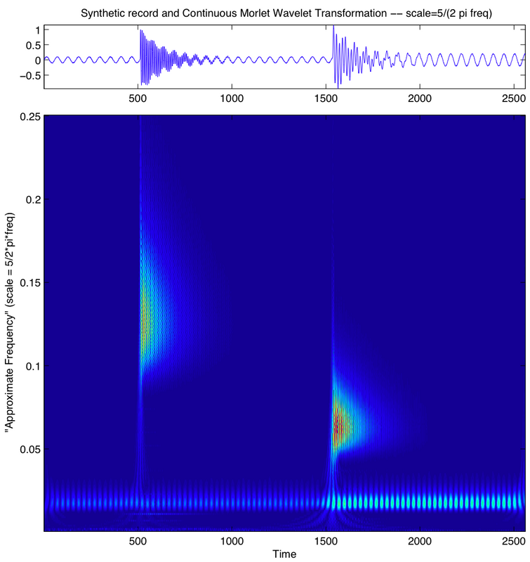
 | Continuous Wavelet Transform (Morlet Wavelet)
[UPDATED]: The previous wavelet image (here) was strongly oscillatory due to an improper choice of arguments during the Wavelet transform. Note: This was my first choice for an overlay filter, but as seen here, the energy of this distribution is unevenly distributed around the known energy of the signal, biased towards higher frequencies. The wavelet scalogram, in general, provides excellent temporal resolution -- unfortunately interpreting the frequency content at each instant is not trivial, and the results are less clear than other methods such as the RID. |
 | Continuous Wavelet Transform (Morlet Wavelet) log10(abs( )) |
 | WVD Filtered with Scalogram as 2-D Overlay Filter
(Morlet Wavelet - Continuous Wavelet Transform) This does not remove some of the serious interference terms, as the WVD contains extreme cross term oscillations in the "interesting" region of the signal. In general, other methods (such as the RID, CW, ZAM) reduce cross-term interference first, within the kernel of the transformation, leading to a better representation. (eg. the log10 plots of the distributions above -- RID, Choi-Williams, ZAM -- while not perfect, do a very good job of removing the cross-term interference.) |
 | WVD Filtered with Scalogram as 2-D Overlay Filter
(Morlet Wavelet - Continuous Wavelet Transform) log10(abs( )) to show the location of energy. |
 | Spectrogram This was obtained using a continous spectrogram implementation, to obtain a point-for-point frequency estimation. This method still falls prey to the time/frequency resolution tradeoff of the typical coarse resolution spectrograms that I've presented before. The windowing involved with creating the STFT by definition smears the arrival of transient signals by a timespan proportional to the windowing function. You can see here that the transient signals appear in the TF plane before the actual time of their onset. |
 | Spectrogram
log10 to show distribution of energy, absolute value not necessary as the spectrogram is entirely non-negative. |
 | WVD Filtered with Spectrogram as 2-D Overlay Filter
This distribution has many of the characteristics that we want from an ideal Time-Frequency representation. Using the spectrogram somewhat removes the interference from so-called "cross terms" (which refers to the cross terms of the quadratic kernel of the WV). The spectrogram is small but nonzero in the regions of interference, and the interference terms of the WVD tend to have double the amplitude of the signal, so this method does not properly address the source of the interference, as seen below where I present the log amplitude. This representation still has negative values, from the interference terms -- eliminating these terms was one of the motivations for trying these types of methods. |
 | WVD Filtered with Spectrogram as 2-D Overlay Filter
log10(abs( )) to show distribution of energy -- in summary this method isn't the best way to address the interference terms in the WVD, there is still a significant amount of energy at the location of the cross-term interference. |
For further references, please refer to the [Main TFR Page].
|